Hyper-connections & what they mean for interpretability

Deepseek's new (viral) mHC paper kickstarted 2026 and brought attention to one of the few meaningful innovations to an LLM's residual stream that we've seen in recent years: Hyper-Connections!

but first: what is the residual stream?

Large language models are made up of a sequence of transformer blocks that continuously "build" the output!

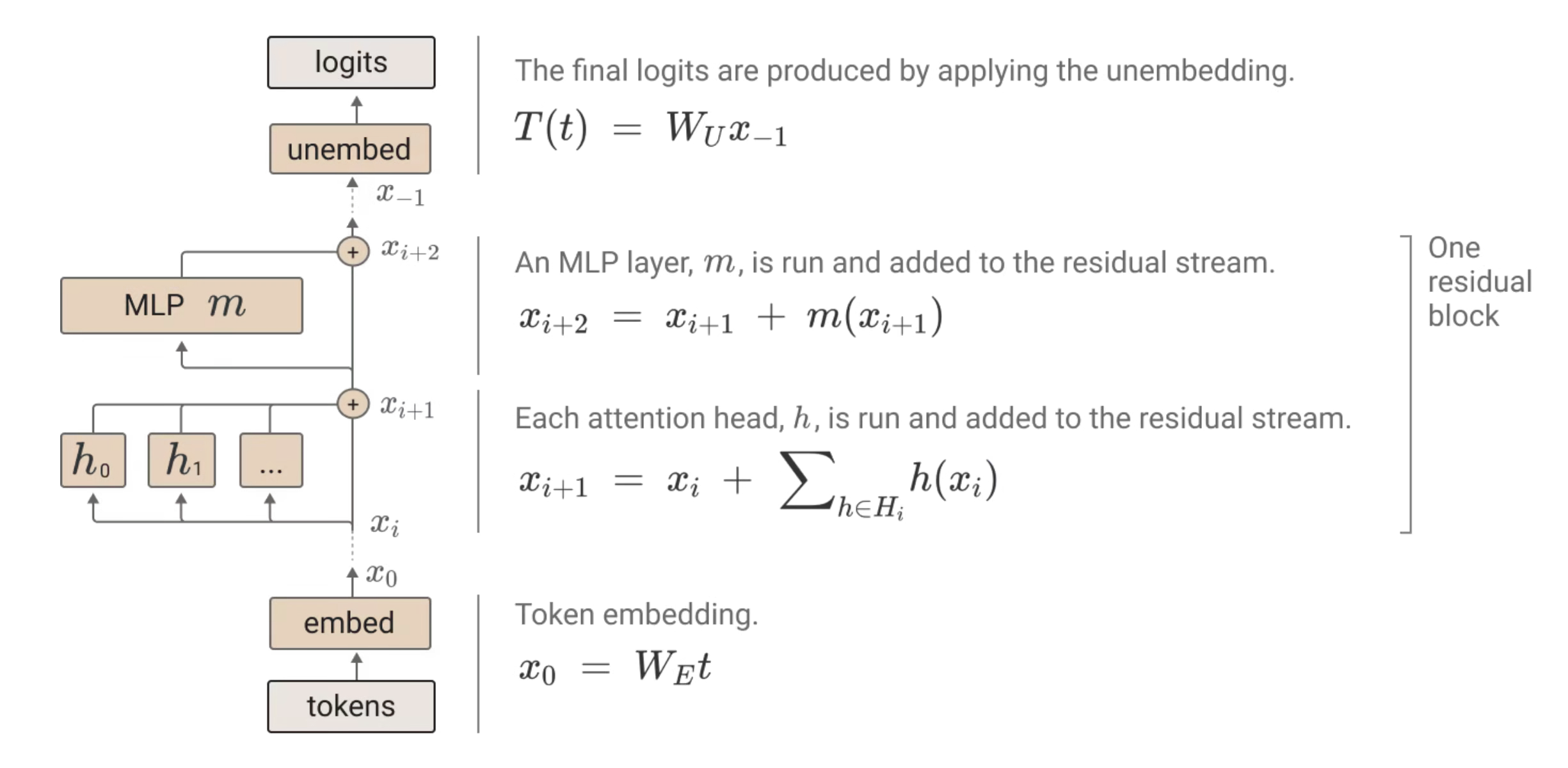(Image from Anthropic)¹

Each block, and each component of each block, reads and writes from the residual stream. This is the communication highway that allows every part of the model to learn (with little-to-no penalty for increasing model lengths).

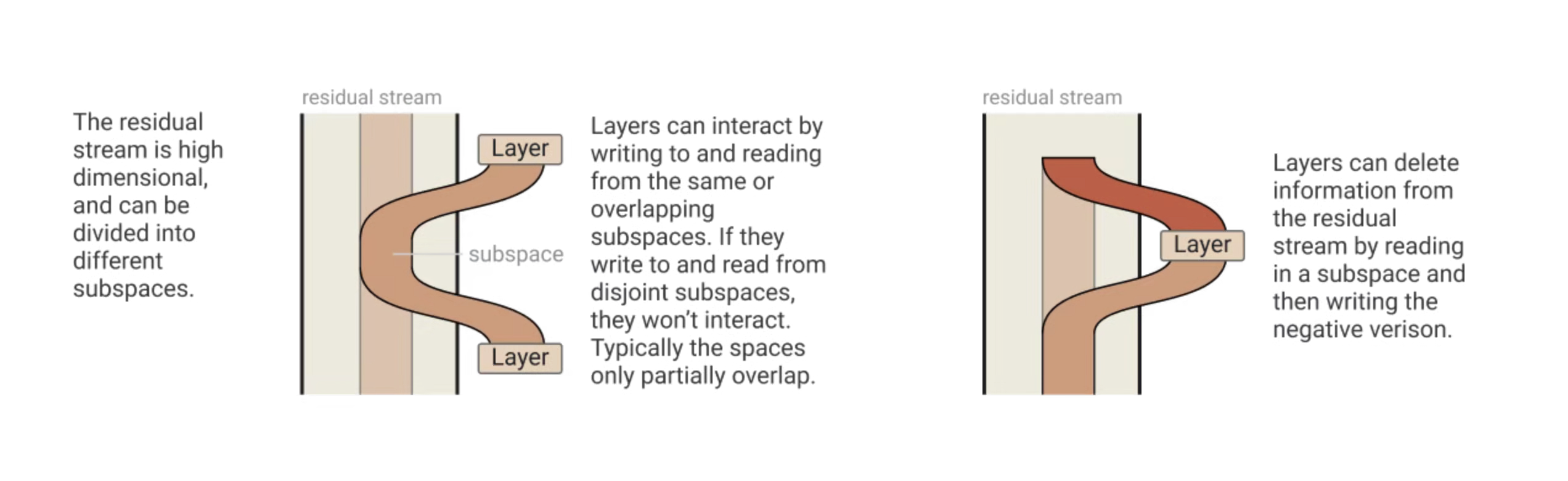(Image from Anthropic)¹

I like to compare this to a factory assembly line. In an assembly line, workers and robots contribute to the end product (say, a car) sequentially. On top of this, each section of workers gets reports on their progress/quality based on the car that ends up being sent to some quality assurance check.

LLMs work surprisingly similarly! Each transformer block of the model is constantly taking things off of the assembly line, adding to it, and putting things back onto the assembly line. The loss function then sends gradient signals to every "worker" (part of the model) telling them how they did!

what are hyper-connections?

Hyper-connections are an architectural addition made by Bytedance (yay tiktok :D) that, instead of using one single residual stream from the previous layer to the remaining ones, uses "multiple streams" meant to allow for more information transfer in more directions.

The idea is best explained by this graphic from Zhu et al.'s paper ².

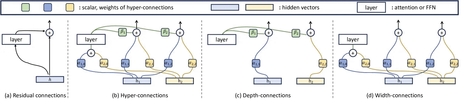
First, you'll notice that HC introduces multiple $\text{hidden vectors}$ ($h \text{ becomes } h_1, h_2, ..., h_n$). This is the model expanding the input into $n$ copies creating a "hyper-hidden matrix". Hyper-connections introduce more lanes for information to travel through!

• Depth-connections ($c$) are like normal residual connections between layers, but with weighting.
• Width-connections ($d$) are residual connections laterally between the $n$ hidden vectors. They also have weighting!

For a single layer, this can be defined as:

The most fun part about this architecture is that it allows the model layers to work in even more parallel than they already do!

Parallelization

In a standard LLM, each layer must wait on the previous layer to compute something before it can continue. This is because layer $n$'s input is layer $(n-1)$'s output.

In hyper-connections, the network learns a routing matrix; that is, a matrix that determines how much information flows from one layer to another. Specifically, this means the model is learning individual weights for each connection between layers. In practice, the model can now do things like 0 out an entire connection (skip a layer) and allow the next layer to start processing "at the same time".

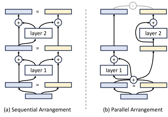
The paper calls this "Sequential-Parallel Duality". It shows that by just changing the values in the Hyper-Connection matrix, the network can switch between a sequential and a parallel structure.

BOOM

The biggest problem with this architecture is that hyper-connection signals, in practice, keep exploding.

The classical residual stream ($y = x + f(x)$) maintains that the model is only copying $1 \cdot x$ when adding it to $f(x)$. The problem with hyperconnections is that they ignore this entirely. It's not longer as simple as adding $x$ to the output of the next layer! The model is learning its own weights/coefficients to boost/reduce connections between layers.

To contrast from the formal single-layer definition of hyper-connections from earlier, here's what it might look like between two or more layers:

Where $L$ and $l$ are a further layer and a previous layer, respectively. Pay close attention to the first term:

$\left(\prod_{i=1}^{L-l} \mathcal{H}_{L-i}^{\mathrm{res}}\right)$ is saying in order to get the signal to the last layer of the network, you have to multiply by every matrix in-between. If the average scaling that each matrix in-between is just a small about like 1.05x or 1.1x, you're failing to preserve the global mean; resulting in unbounded growth.

In other words, the model can learn that it needs to boost a connection by 1.1x every layer, and by layer 100, that's a 1,378,061% increase in residual stream values! This can lead to loss spikes, exploding gradients, and a bunch of other training issues that would be extremely hard to diagnose.

---

the solution: manifold-constrained hyper-connections

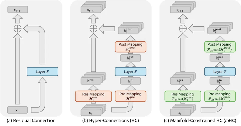
Deepseek builds on Bytedance's hyper-connections with manifold-constrained hyper-connections.³

first: what is a manifold?

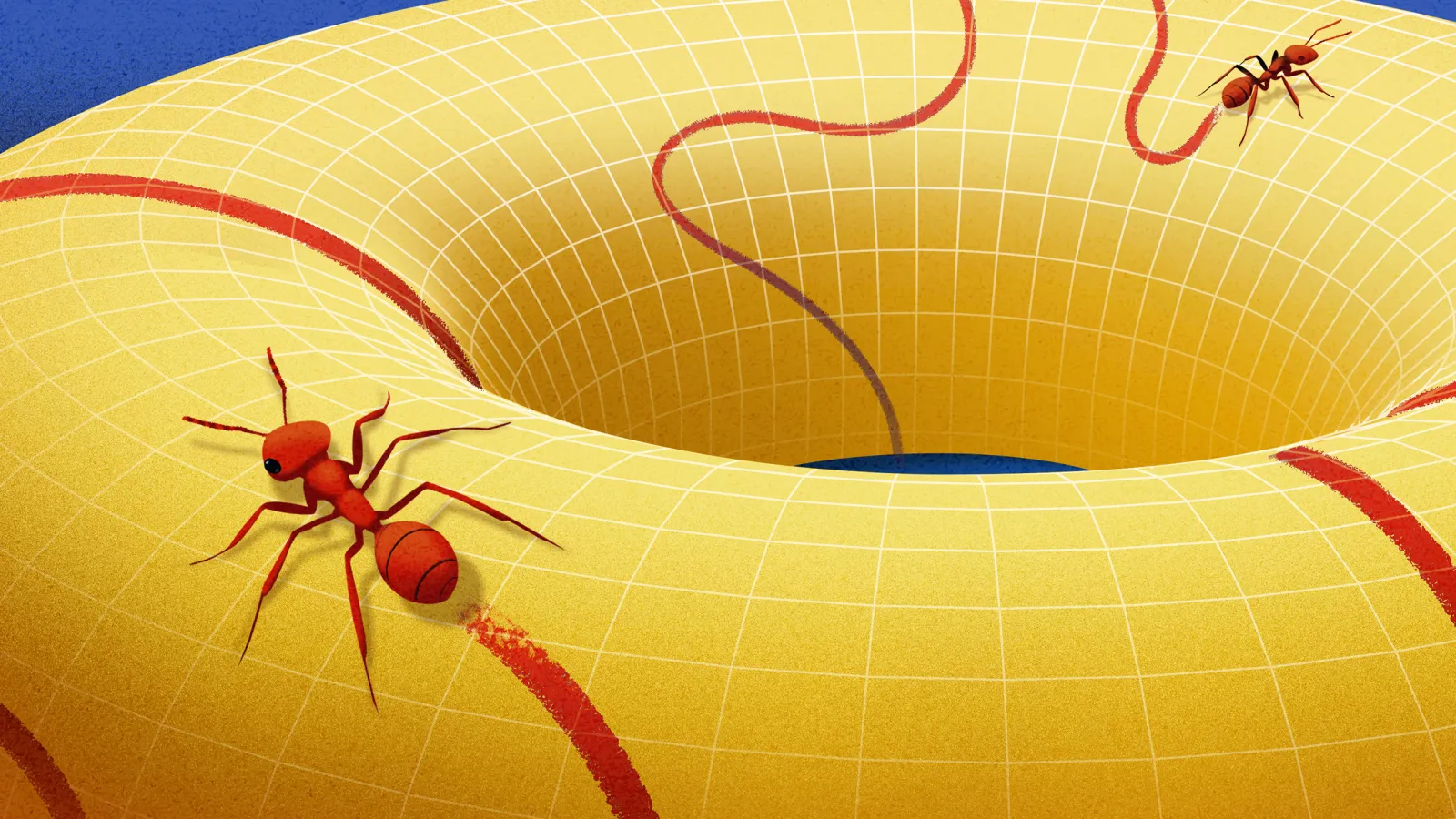(Image from Quanta Magazine⁴)

When you think of "mathematical space", you might first think of the euclidean plane, or a number line! This is where the coordinate system allows for trigonometry, calculus, and more.

But what if that plane took a different shape? What if it were curved? How does the math we've developed for centuries transfer when two points have inconsistent distances, parallel lines can intersect, and the normal rules have been turned upside down?

Enter, the manifold:

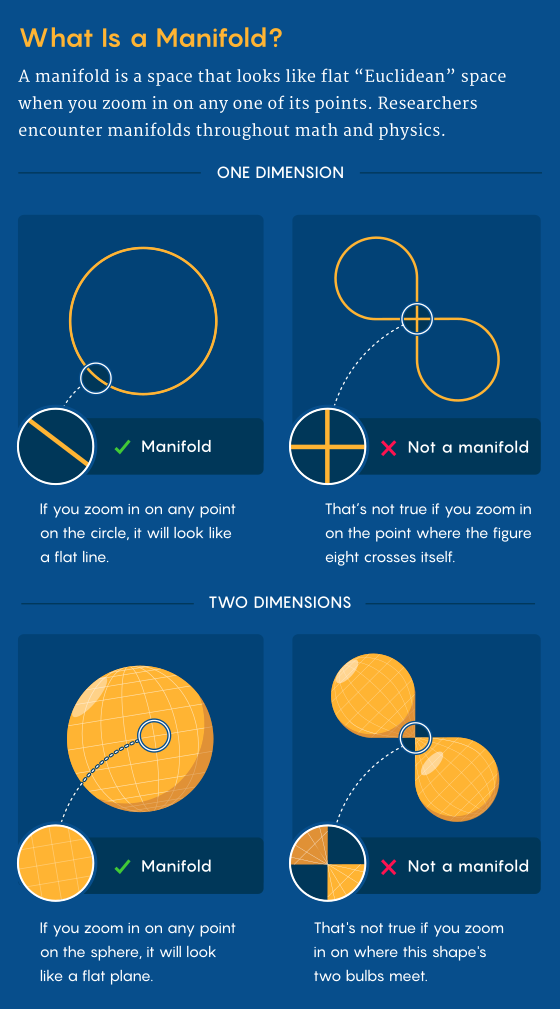(Image from Quanta Magazine⁴)

A manifold is a space that might be curved or twisted globally, but looks flat if you zoom in far enough. This property is called being locally Euclidean.

The easiest way to think about local euclideanity(?) is to think about the Earth's surface! It's a sphere, but from wherever you're standing it looks flat.

Some other examples of manifolds:

• A sphere (2D manifold in 3D space): Every point on the surface locally looks like a flat plane
• A torus (donut): Also locally flat, despite its global curvature
• A Mobius strip: Locally flat, but globally has only one side!
• Even a plain old flat plane is technically a manifold (just a boring one)

The key insight is that manifolds give us a way to do calculus on curved surfaces. Since every small patch is essentially flat, we can use all our familiar tools—derivatives, gradients, optimization—by working locally. This is the foundation of a subfield called differential geometry.

constraining hyper-connections to a manifold

As I said above, the problem with hyper-connections was that the model was learning connection weights of any size. These could be miniscule but were often huge.

Deepseek found that in order to constrain the values to a specific size, they could restrict the values to fit in a single manifold. The idea here is to make sure that all of the information is flowing along a "well-behaved" surface. Instead of letting connection weights $w_{\text{all}} \in \mathbb{R}^n$, we constrain them to only values on a manifold with specific properties.

In order to create this limitation, Deepseek defers to the Sinkhorn-Knopp algorithm to project $\mathcal{H}_{l}^{\mathrm{res}}$ onto the Birkhoff Polytope.

aside: holy words.

Sinkhorn-Knopp algorithm: An iterative algorithm that transforms any non-negative matrix into a doubly stochastic matrix. It works by alternating between normalizing rows and normalizing columns until convergence. In mHC, this is used to project the learned routing weights onto a valid doubly stochastic form.

• Doubly Stochastic: A matrix where all entries are non-negative, and every row and every column sums to exactly 1.

Birkhoff Polytope: The set of all $n \times n$ doubly stochastic matrices. It's a convex shape whose corners (vertices) are exactly the permutation matrices. By constraining $\mathcal{H}_{l}^{\mathrm{res}}$ to live on this polytope, Deepseek ensures that connection weights can't explode—each row summing to 1 means outputs are weighted averages, and each column summing to 1 means total signal is preserved across layers! (rather than amplifying or shrinking)

---

interpreting the new residual stream(s)

This segment is a collection of thoughts on how we might go about applying mechanistic interpretability techniques to a model with hyper-connections. It's meant to be (very) preliminary, and I hope to be able to train/get access to such a model and be able to perform experiments on it!

Mechanistic interpretability acts upon the residual stream as the stream of information between layers. If a model now sends information across multiple highways, does this make interpretability harder? or easier?

Without having a model trained with hyper-connections to play around with, we're stuck operating in the hypothetical. The following is essentially a research project proposal/first steps to examine this type of model architecture. I hope that soon I can wrap a model with some interpretability tools and carry out these experiments myself!

more superposition

Classically, mechanistic interpretability methods focus on the output of the residual stream at a given layer. However, MHC introduces even more complexity to the process by splitting the residual stream into parallel streams! This introduces a new challenge one might (in a cliche fashion) call stream superposition: one concept can be split across mulitple residual streams at the same time!

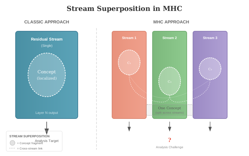(Thank you Claude for the wonderful diagram!)

However, similarly to how Anthropic (somewhat) "resolved" the problem of cross-layer superposition⁵ (assuming faithfulness), we may find fruit in applying the same methodology to the split residual stream and reading from/writing to all streams at once.

We might call this approach a cross-stream transcoder:

Consider a model with $n$ parallel residual streams at each layer. Let $\mathbf{x}_l^{(i)} \in \mathbb{R}^d$ denote the activation of stream $i$ at layer $l$, where $d$ is the model dimension. We concatenate all streams into a single tensor:

A cross-stream transcoder (CST) consists of an encoder $\mathcal{E}$ and per-stream decoders $\mathcal{D}^{(i)}$. The encoder maps the concatenated streams to a sparse latent representation:

where $\mathbf{W}_{\text{enc}} \in \mathbb{R}^{m \times nd}$ is the encoder weight matrix, $\mathbf{b}_{\text{enc}} \in \mathbb{R}^m$ is the encoder bias, and $m$ is the (overcomplete) dictionary size. The JumpReLU nonlinearity enforces sparsity in the latent activations.⁶

For MLP replacement, each stream's output is reconstructed via stream-specific decoders:

where $\mathbf{W}_{\text{dec}}^{(i)} \in \mathbb{R}^{d \times m}$ reconstructs the MLP contribution to stream $i$.

The training objective combines reconstruction fidelity across all streams with a sparsity penalty:

where $\mathbf{y}_l^{(i)}$ is the true MLP output for stream $i$, $\mathbf{W}_{\text{dec}, j}$ denotes the $j$-th column across all decoder matrices, and $\lambda, c$ are hyperparameters controlling sparsity.

intuition

The key property of the CST is that a single latent concept $a_{l,j}$ can contribute to multiple streams simultaneously through its decoder weights $\mathbf{W}_{\text{dec},j}^{(1)}, \ldots, \mathbf{W}_{\text{dec},j}^{(n)}$. This directly addresses stream superposition: if a concept is distributed across, say, streams $\{2, 3\}$, the CST can learn a single sparse feature that writes to exactly those streams with appropriate magnitudes, recovering the unified representation that the architecture had fragmented.

This mirrors how crosscoders resolve cross-layer superposition by jointly encoding multiple layers⁵, but applied to cross-stream superposition within a single layer.

accounting for dynamic routing

The formulation above treats the residual streams as static highways. However, HC/mHC's routing matrices $\mathcal{H}_l^{\text{res}}$ are input-dependent: they dynamically gate which streams propagate to subsequent layers. A feature present in stream $i$ at layer $l$ may be ablated if the routing matrix zeroes out that pathway.

To account for this, we define the effective transmitted activation for feature $j$:

where $\mathcal{H}_l^{\text{res}}[i, i']$ is the routing weight from stream $i$ to stream $i'$ at layer $l$. This captures how much of feature $j$'s contribution to stream $i$ actually reaches stream $i'$ in the next layer.

The total effective activation of feature $j$ arriving at stream $i'$ in layer $l+1$ is then:

This means interpreting CST latents requires examining them jointly with the instantaneous routing state. A feature might be "active" in the CST sense ($a_{l,j} > 0$), but functionally silent if the routing matrix blocks its transmission pathways.

caveat

However, this could be completely wrong! I think I'd need both a better fundamental mathematical intution for what hyper-connections do for model learnings and to actually play around with a model to see if there is actually any cross-stream superposition!

new observables for interpretability

Some good news though: the HC/mHC papers introduce specific visualizations that can serve as new high-level interpretability tools:

Connection Matrices ($C^{(i)}$): The paper visualizes the unfolded dependency of layer outputs on previous layers. This lets researchers immediately see the "effective architecture" that the model has learned:

• A vertical strip in the matrix indicates a layer that contributes to all future layers—a "global broadcaster" that's computed once and reused everywhere downstream
• A diagonal pattern indicates local processing, where each layer primarily influences only its immediate neighbors

A-Shaped Connection Patterns: The papers observe a characteristic "A-shaped" pattern in the connection matrices. This combines:

• Long-term decay (Post-Norm style): Later layers gradually rely less on much earlier layers
• Frequent access to bottom layers (Pre-Norm style): Even deep layers maintain strong connections back to the earliest layers

The implication here is fascinating: the model automatically learns a hybrid architecture that combines the best properties of both Pre-Norm and Post-Norm transformers. We can analyze this shape to determine which early-layer features (e.g., positional embeddings or induction tokens) are being "cached" for long-term use throughout the forward pass.

Footnotes

1. A mathematical Framework for Transformer Circuits (Elhage et al.) ↩ ↩²

2. Hyper-Connections (Zhu et al.) ↩

3. Manifold-Constrained Hyper-Connections (Xie et al.) ↩

4. What Is a Manifold? (Paulina Rowińska for Quanta Magazine) ↩ ↩²

5. Sparse Crosscoders for Cross-Layer Features and Model Diffing (Lindsey et al.) ↩ ↩²

6. Scaling and Evaluating Sparse Autoencoders (Gao et al.) ↩