Exploring how transformers represent dataset geometry
Can transformers learn geometric information about a dataset? Maybe! I briefly explain one framework to reason about this using transformers and a toy dataset, and then dive into some experiments building ontop of it.
Large language models are a tangled web of different internal mechanisms that represent the model's training process over a large dataset. What if we knew some geometric fact about the dataset? Does the model learn the same geometry internally? Simplex says that they do!
Simplex?
Paul Riechers and Adam Shai (Simplex Research) set off to understand if a transformer can learn its dataset's "belief state geometry".
Their setup:
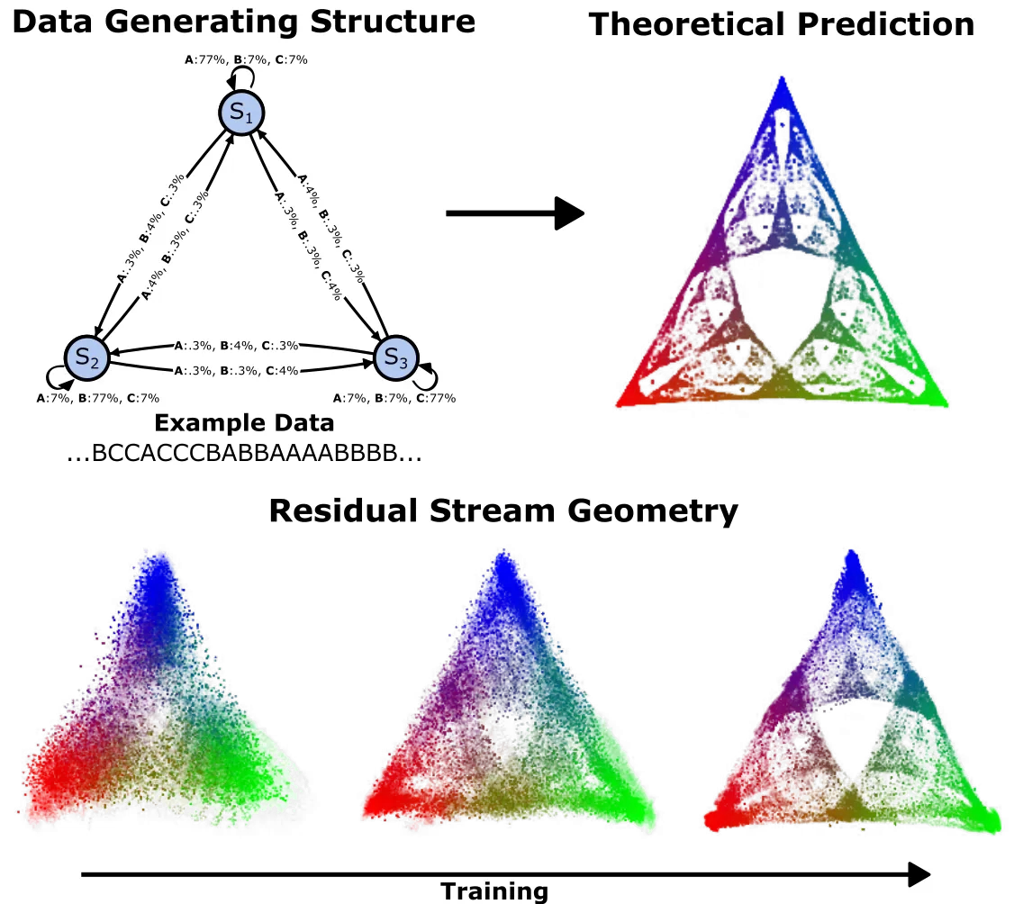
If you sample data from a Hidden Markov Model, you can calculate a ground truth vector: a probability distribution over the future states given the observed history.
For an HMM with three states, these belief vectors projected onto a 2-simplex trace out a fractal geometry that you can determine by tweaking the HMM's parameters. Shai et al., 2024 show that if you train a transformer on data generated by the emissions of such HMMs the model can internally reconstruct the geometric structure presented on the 2-simplex!
The following is the result of a research sprint I did as a test task for Simplex's MATS Stream! It involved understanding what happens when the data you train the transformer on comes from a mixture of HMMs. We expect the model to have to do two things at once:
- figure out which process generated the sequence
- track the belief state within that process
The setup
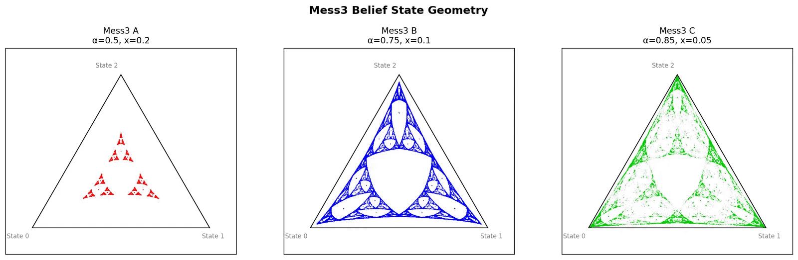
I set up 3 Mess3 processes for the training dataset.
| Process | ||
|---|---|---|
| Mess3 A | 0.50 | 0.20 |
| Mess3 B | 0.75 | 0.10 |
| Mess3 C | 0.85 | 0.05 |
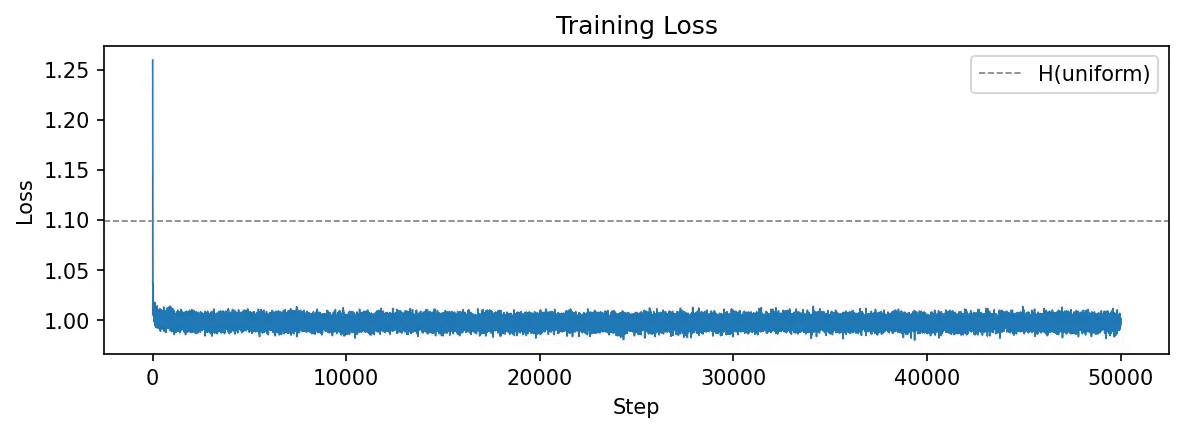
I then train a 2 layer Transformer model (, 4 heads, , context length 12) for 50k steps with batch size 2048 and Adam (, no weight decay).
How is this type of structure relevant to language models?
Pretend you're a language model (or, just a human) and you see the token "i". At first, you don't really know what "i" means. However, after you see another token, such as "i love" you know that you're reading something related to love or endearment! If you saw "i in range" you'd know you're reading code.
Our 3-Mess3 mixture works the same way. All three processes emit from the same vocabulary , but with different transition and emission statistics. The model has to figure out which Mess3 it's looking at and track the belief state within that process. Token in Mess3 A means something different than the same token in Mess3 B.
My Prediction
I predicted that the residual stream would organize into three orthogonal subspaces (one per Mess3 component). Why?
We can write the non-ergodic mixture as a single block-diagonal GHMM with 9 latent states (3 per Mess3 component). Before seeing any tokens, the predictive vector is uniform over all 9 states.
Because is block-diagonal, the three components' latent states never interact. The predictive vector decomposes as:
where are posterior component weights (they sum to 1) and each is the within-component belief. The weights update via Bayes' rule:
and each within-component belief updates independently with its own transition matrix.
The block-diagonal transitions keep these subspaces from ever interacting:
So the ground truth vectors already sit in three orthogonal subspaces of . We should be able to find each of these individual structures by probing the residual stream, just like Shai et al., 2024 does for one HMM.
This is related to the factored world hypothesis1, but there's a key difference. In their paper, simultaneous independent factors live in a tensor-product latent space (), and transformers discover the factorization, compressing exponential dimensionality down to linear. Our setup is simpler: the latent space is already a direct sum, and the orthogonal structure is baked into the data generator. I was predicting the transformer would preserve a factorization that's already there, rather than discovering a hidden one.
Residual Stream Geometry Analysis
I trained a linear probe on the residual stream, and found that it recovered each Mess3's belief geometry separately.
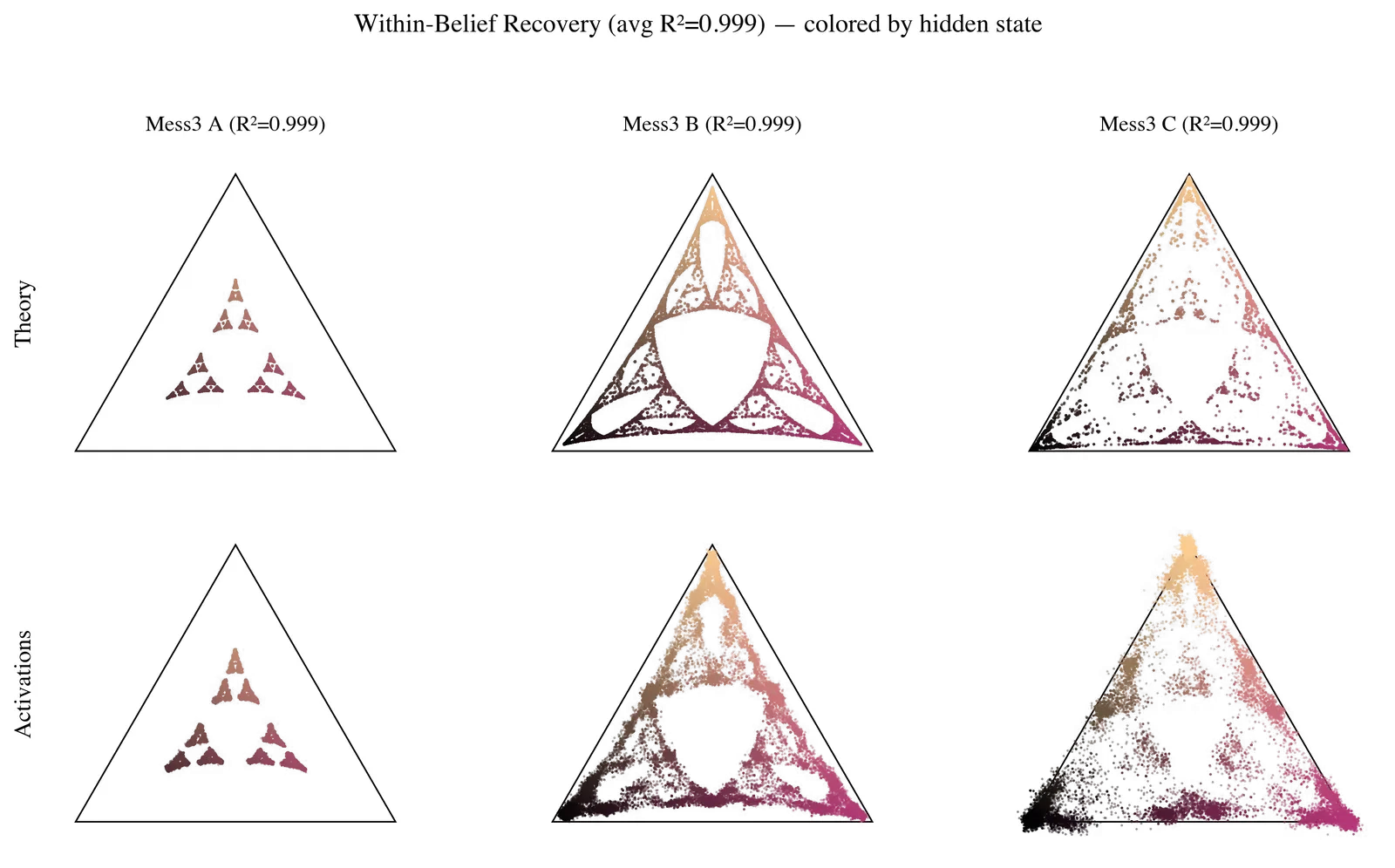
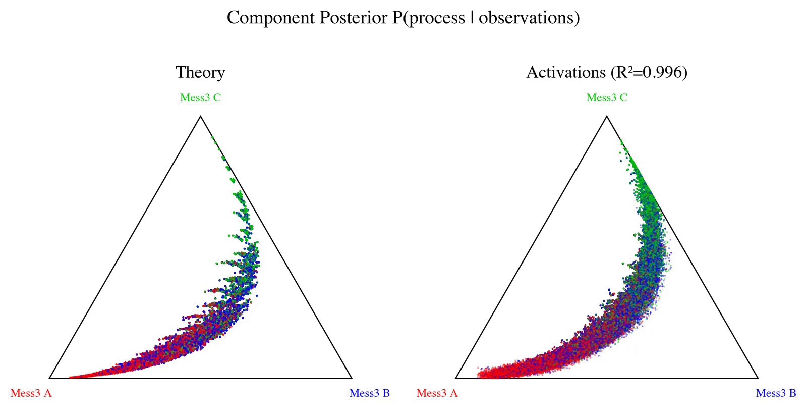
The model also encoded the geometry representing which Mess3 generated the sequence. I regressed from activations to the full 9D joint belief vector and marginalized over within-component states, which gave me the component posterior on the 2-simplex.
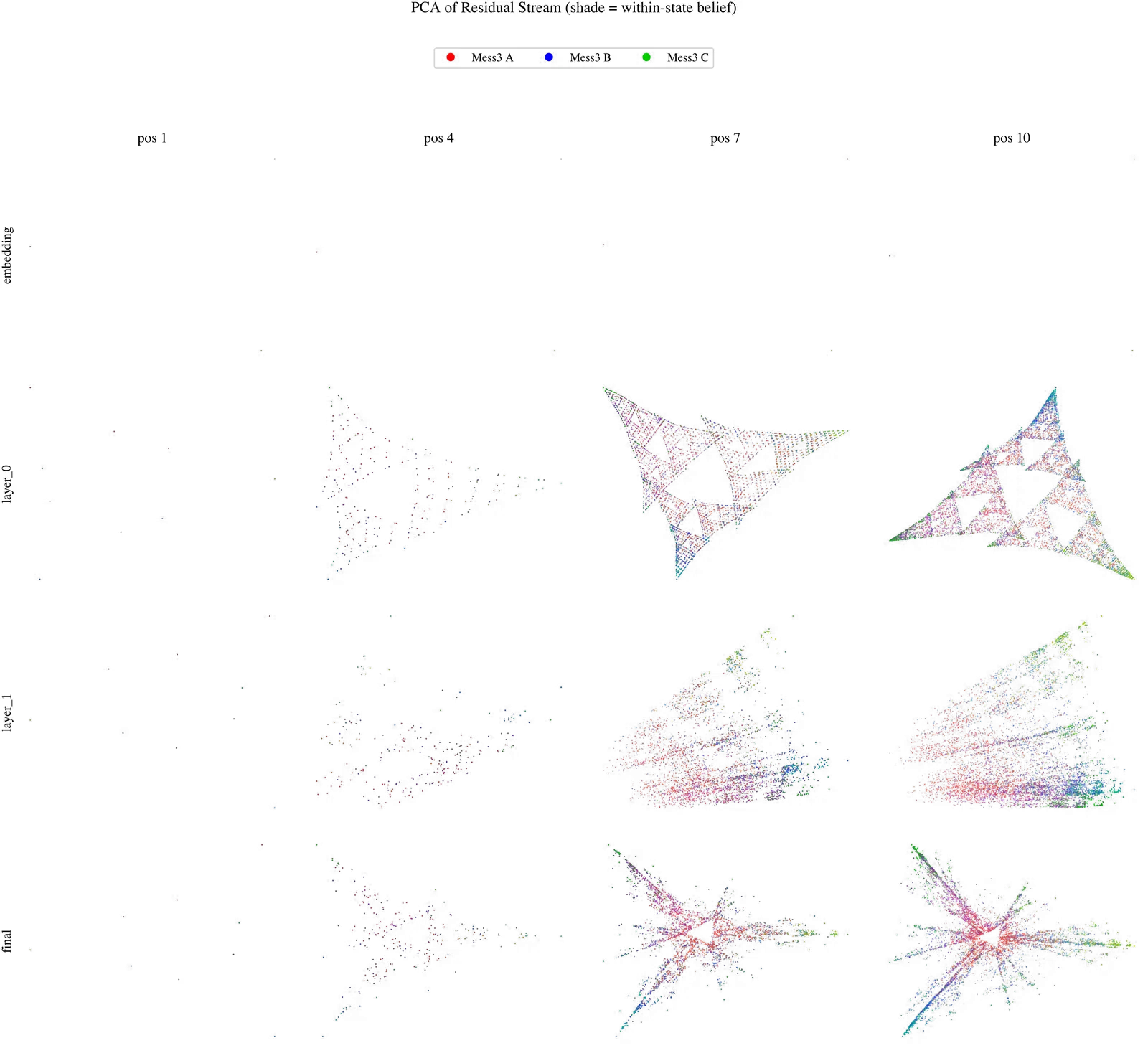
I ran PCA on the residual stream activations, coloring each point by process identity (hue) and within-state belief (shade). At the embedding layer, you can only see the three discrete token identities. After layer 0, fractal simplex-like structure started showing up, but the three processes still overlapped in PC space. By the final layer at later positions, the three clusters fully separated, and each one contained its own internal belief simplex. The residual stream geometry pointed towards three copies of the 2-simplex sitting in .
Orthogonality
I originally predicted three mutually orthogonal subspaces (one per component). To test this, I fit linear probes to each and checked cross-subspace prediction: could process 's beliefs be recovered from process 's probe subspace?
Looking across all layers concatenated, A's subspace was orthogonal to B and C (cosines ). B and C, on the other hand, heavily overlapped (cosines up to 0.97). That tracked: Mess3B & Mess3C have similar parameters!
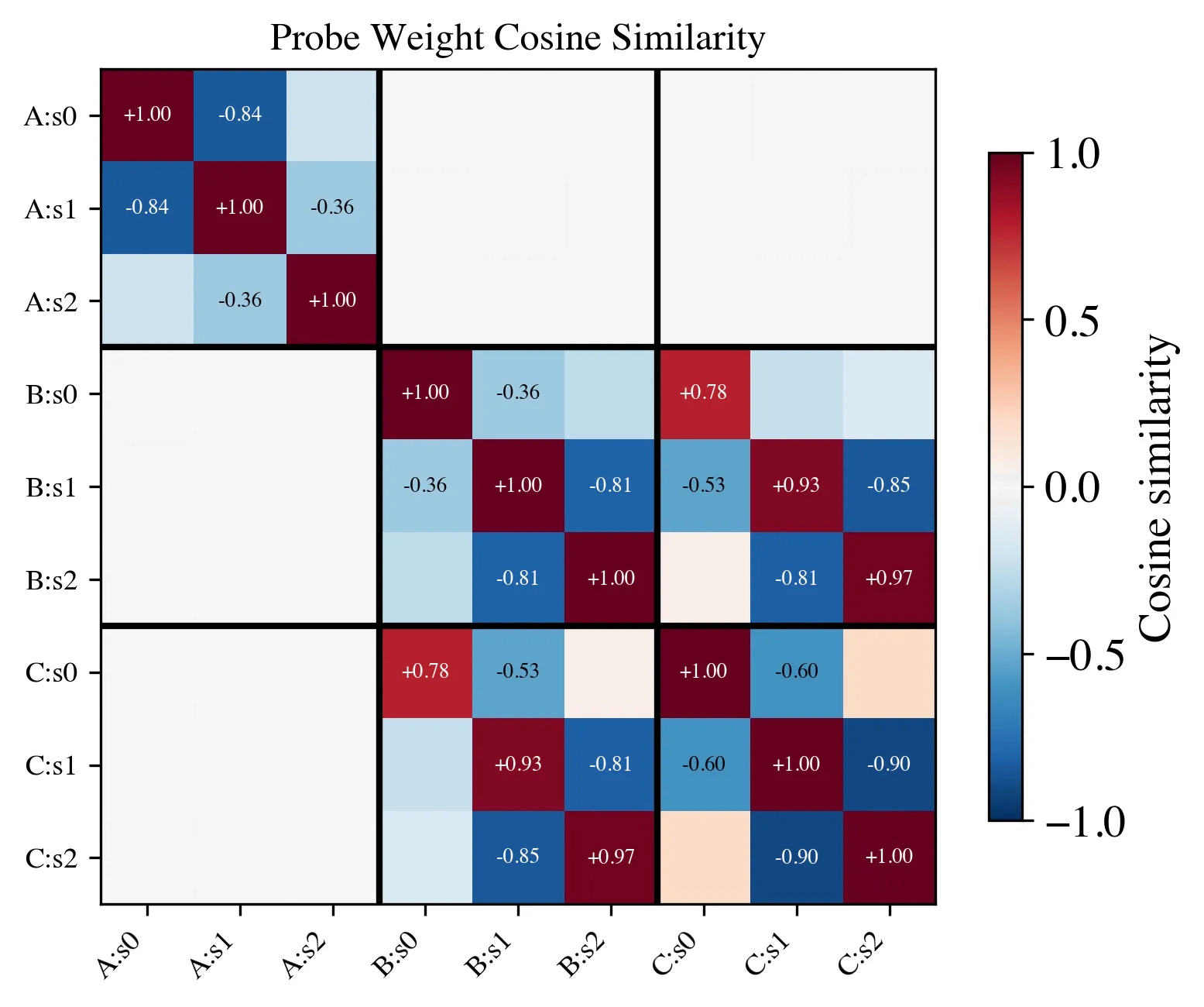
So, in the end, my block-diagonal prediction was half right! A got its own subspace. B and C shared directions instead of maintaining separate ones.
Conclusion
This was one of the most exciting research sprints I've done in a while! I think it was extremely interesting to dive into computational mechanics for a weekend, and learn about the factored world that Paul and Adam live in. Understanding model belief states will be increasingly important as we move towards an age where it might be time to start tracking LLM goal/belief states via evaluations in the future!
Footnotes
-
Shai et al., "Transformers Represent Belief State Geometry in their Residual Stream", 2026. ↩